Coffee Survey

1.Introduction

1.1 Import modules and dataset

import matplotlib.pyplot as plt
import pandas as pd
import plotly.express as px
import seaborn as sns

df = pd.read_csv("../../data_sources/coffee_survey.csv")

1.2 Data Exploration

df.head(10)

	Unnamed: 0	age	cups	where_drink	purchase_other	favourite	favorite_specify	additions	additions_other	sweetener	...	most_paid	most_willing	value_cafe	spent_equipment	value_equipment	gender	education_level	employment_status	number_children	political_affiliation
0	1	<18 years old	3	At home, At the office, At a cafe	NaN	Pourover	NaN	No - just black, Milk, dairy alternative, or c...	NaN	NaN	...	NaN	NaN	NaN	NaN	NaN	Other (please specify)	Bachelor's degree	Employed full-time	More than 3	Democrat
1	2	>65 years old	3	At the office, At a cafe	NaN	Cortado	NaN	No - just black	NaN	NaN	...	NaN	NaN	NaN	NaN	NaN	NaN	NaN	NaN	NaN	NaN
2	3	25-34 years old	1	At home, At the office, On the go	NaN	Regular drip coffee	NaN	Milk, dairy alternative, or coffee creamer, Su...	NaN	Granulated Sugar, Brown Sugar	...	NaN	NaN	NaN	NaN	NaN	Female	Bachelor's degree	Employed full-time	NaN	Democrat
3	4	18-24 years old	2	At the office	NaN	Iced coffee	NaN	Milk, dairy alternative, or coffee creamer	NaN	NaN	...	NaN	NaN	NaN	NaN	NaN	NaN	NaN	NaN	NaN	NaN
4	5	45-54 years old	2	At home, At the office, At a cafe, On the go	NaN	Regular drip coffee	NaN	No - just black	NaN	NaN	...	$4-$6	$8-$10	No	$500-$1000	Yes	Male	Master's degree	Employed full-time	2	No affiliation
5	6	>65 years old	1	At home	NaN	Regular drip coffee	NaN	No - just black	NaN	NaN	...	NaN	NaN	NaN	NaN	NaN	NaN	NaN	NaN	NaN	NaN
6	7	25-34 years old	2	At home, At the office	NaN	Pourover	NaN	No - just black	NaN	NaN	...	$2-$4	More than $20	Yes	$50-$100	Yes	Male	Master's degree	Unemployed	NaN	Independent
7	8	35-44 years old	1	At the office, At home	NaN	Iced coffee	NaN	No - just black	NaN	NaN	...	$10-$15	More than $20	Yes	$100-$300	Yes	Male	Bachelor's degree	Employed full-time	3	No affiliation
8	9	45-54 years old	More than 4	At home	NaN	Pourover	NaN	No - just black	NaN	NaN	...	$10-$15	$15-$20	Yes	$300-$500	Yes	Male	Bachelor's degree	Employed full-time	3	No affiliation
9	10	35-44 years old	1	At the office, At a cafe, At home	NaN	Cappuccino	NaN	Milk, dairy alternative, or coffee creamer, Su...	NaN	Granulated Sugar, Brown Sugar	...	NaN	NaN	NaN	NaN	NaN	NaN	NaN	NaN	NaN	NaN

10 rows × 43 columns

Age exploration

sns.catplot(data = df, x = "age", kind="count", height=5, aspect=2)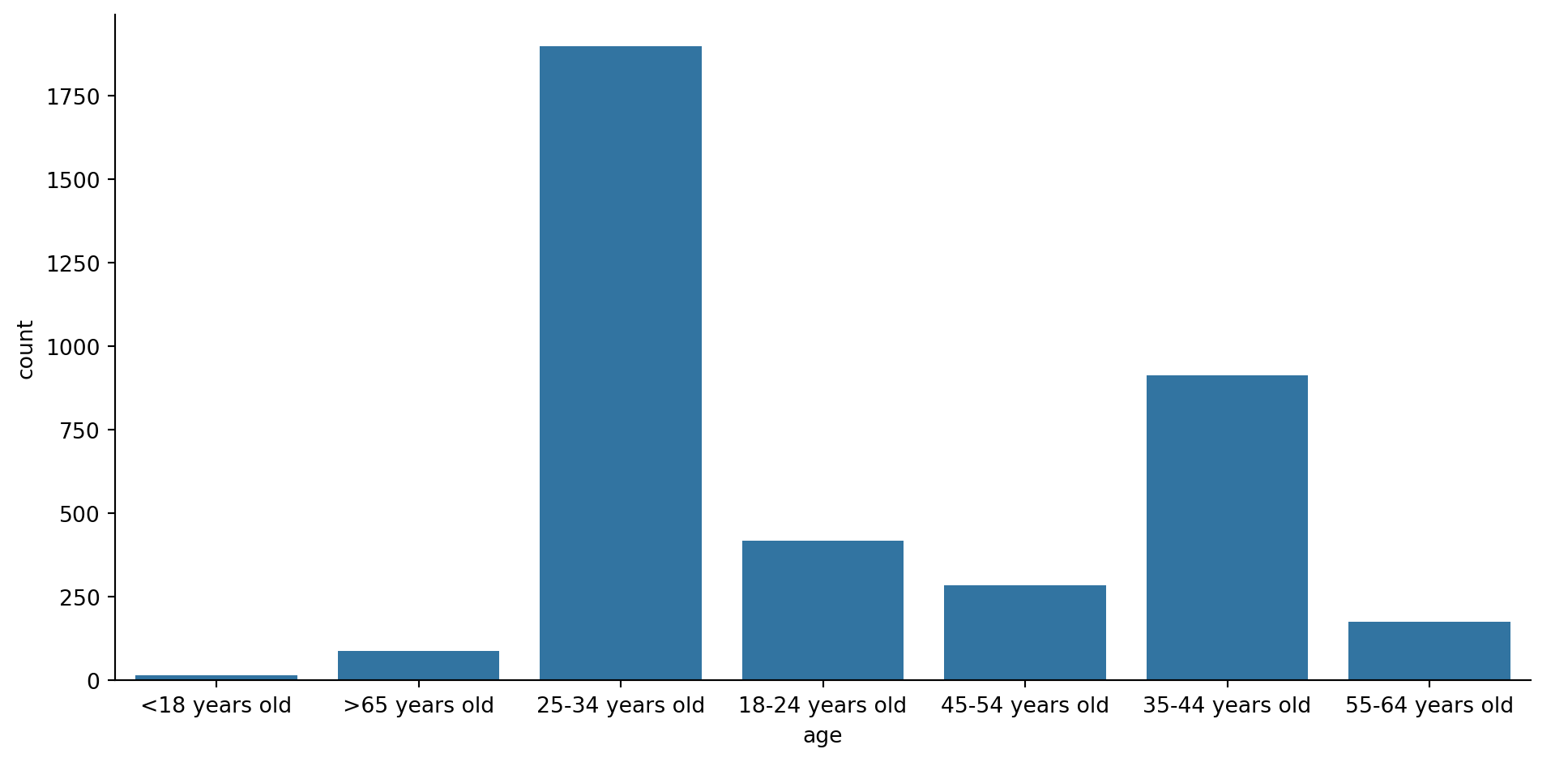

• Age 25 to 34 range is the highest age range among coffee customers.

1.3 Data Filtering

df_focused = df[["age", "where_drink", "favourite", 'style']].copy()
df_focused.head(10)

	age	where_drink	favourite	style
0	<18 years old	At home, At the office, At a cafe	Pourover	Bright
1	>65 years old	At the office, At a cafe	Cortado	Fruity
2	25-34 years old	At home, At the office, On the go	Regular drip coffee	Sweet
3	18-24 years old	At the office	Iced coffee	Nutty
4	45-54 years old	At home, At the office, At a cafe, On the go	Regular drip coffee	Floral
5	>65 years old	At home	Regular drip coffee	Full Bodied
6	25-34 years old	At home, At the office	Pourover	Floral
7	35-44 years old	At the office, At home	Iced coffee	Fruity
8	45-54 years old	At home	Pourover	Full Bodied
9	35-44 years old	At the office, At a cafe, At home	Cappuccino	Nutty

• Focusing on 4 attributes including age, where to drink, favourite, and style of drinking coffee.

2. Data Analysis

2.1 Preferred Coffee Places by Age Group

#Manage “where_drink” : spliting words

df_focused['where_drink'] = df_focused['where_drink'].fillna('')
df_focused['where_list']=df_focused['where_drink'].str.split(pat=", ")
df_focused.head()

	age	where_drink	favourite	style	where_list
0	<18 years old	At home, At the office, At a cafe	Pourover	Bright	[At home, At the office, At a cafe]
1	>65 years old	At the office, At a cafe	Cortado	Fruity	[At the office, At a cafe]
2	25-34 years old	At home, At the office, On the go	Regular drip coffee	Sweet	[At home, At the office, On the go]
3	18-24 years old	At the office	Iced coffee	Nutty	[At the office]
4	45-54 years old	At home, At the office, At a cafe, On the go	Regular drip coffee	Floral	[At home, At the office, At a cafe, On the go]

#Manage “where_drink” : exploding and making them to list then one-hot for the list

df_exploded = df_focused.explode('where_list')
dummies = pd.crosstab(df_exploded.index, df_exploded['where_list'])
df_final = df_focused.join(dummies.groupby(dummies.index).sum())
df_final.head()

	age	where_drink	favourite	style	where_list		At a cafe	At home	At the office	None of these	On the go
0	<18 years old	At home, At the office, At a cafe	Pourover	Bright	[At home, At the office, At a cafe]	0	1	1	1	0	0
1	>65 years old	At the office, At a cafe	Cortado	Fruity	[At the office, At a cafe]	0	1	0	1	0	0
2	25-34 years old	At home, At the office, On the go	Regular drip coffee	Sweet	[At home, At the office, On the go]	0	0	1	1	0	1
3	18-24 years old	At the office	Iced coffee	Nutty	[At the office]	0	0	0	1	0	0
4	45-54 years old	At home, At the office, At a cafe, On the go	Regular drip coffee	Floral	[At home, At the office, At a cafe, On the go]	0	1	1	1	0	1

#Manage “where_drink” : exploring mean for each group of age

groupby_age = df_final.groupby('age')[df_final.select_dtypes(include='number').columns].mean()
groupby_age.head()

		At a cafe	At home	At the office	None of these	On the go
age
18-24 years old	0.002398	0.414868	0.872902	0.342926	0.016787	0.194245
25-34 years old	0.001055	0.329641	0.912975	0.390295	0.011603	0.188291
35-44 years old	0.001095	0.265060	0.933187	0.369113	0.003286	0.181818
45-54 years old	0.000000	0.161972	0.957746	0.250000	0.000000	0.140845
55-64 years old	0.017045	0.085227	0.948864	0.284091	0.000000	0.102273

#Stacked bar plot

groupby_age.plot(kind='bar', stacked=True, figsize=(10,6), colormap='tab20')
plt.title('Preferred Coffee Places by Age Group')
plt.ylabel('Proportion of Respondents')
plt.xlabel('Age Group')
plt.legend(title='Where People Drink Coffee', bbox_to_anchor=(1.05, 1), loc='upper left')
plt.tight_layout()
plt.show()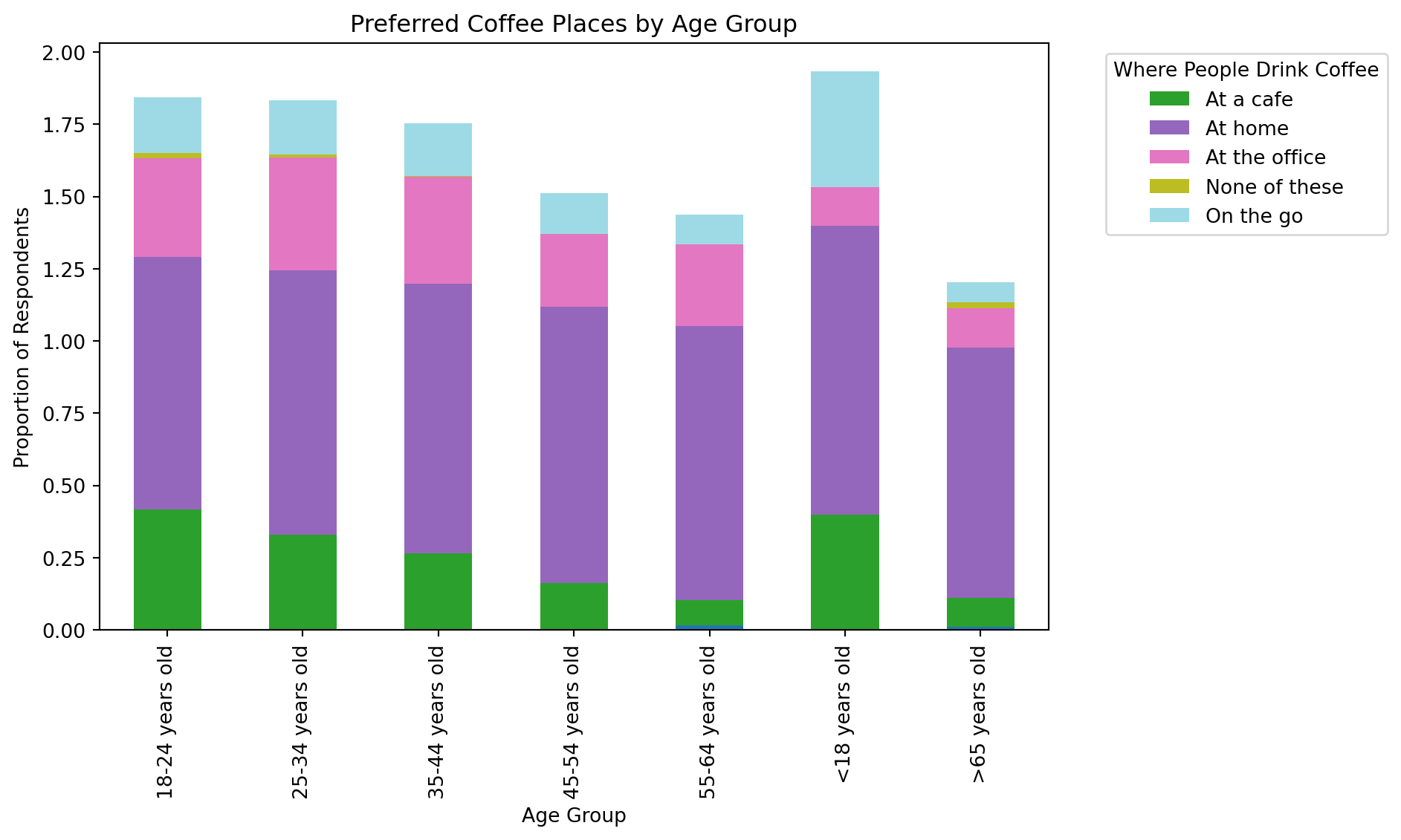

2.2 Preferred Type of Coffee by Age Group

#Group favourite by Age

favourite_by_agegroup = df_focused.groupby('age')['favourite'].value_counts().unstack().fillna(0)

#Heatmap

plt.figure(figsize=(12, 6))
sns.heatmap(favourite_by_agegroup, annot=True, fmt='.0f', cmap='YlGnBu')
plt.title('Favorite Type by Age Group')
plt.ylabel('Age Group')
plt.xlabel('Favorite')
plt.tight_layout()
plt.show()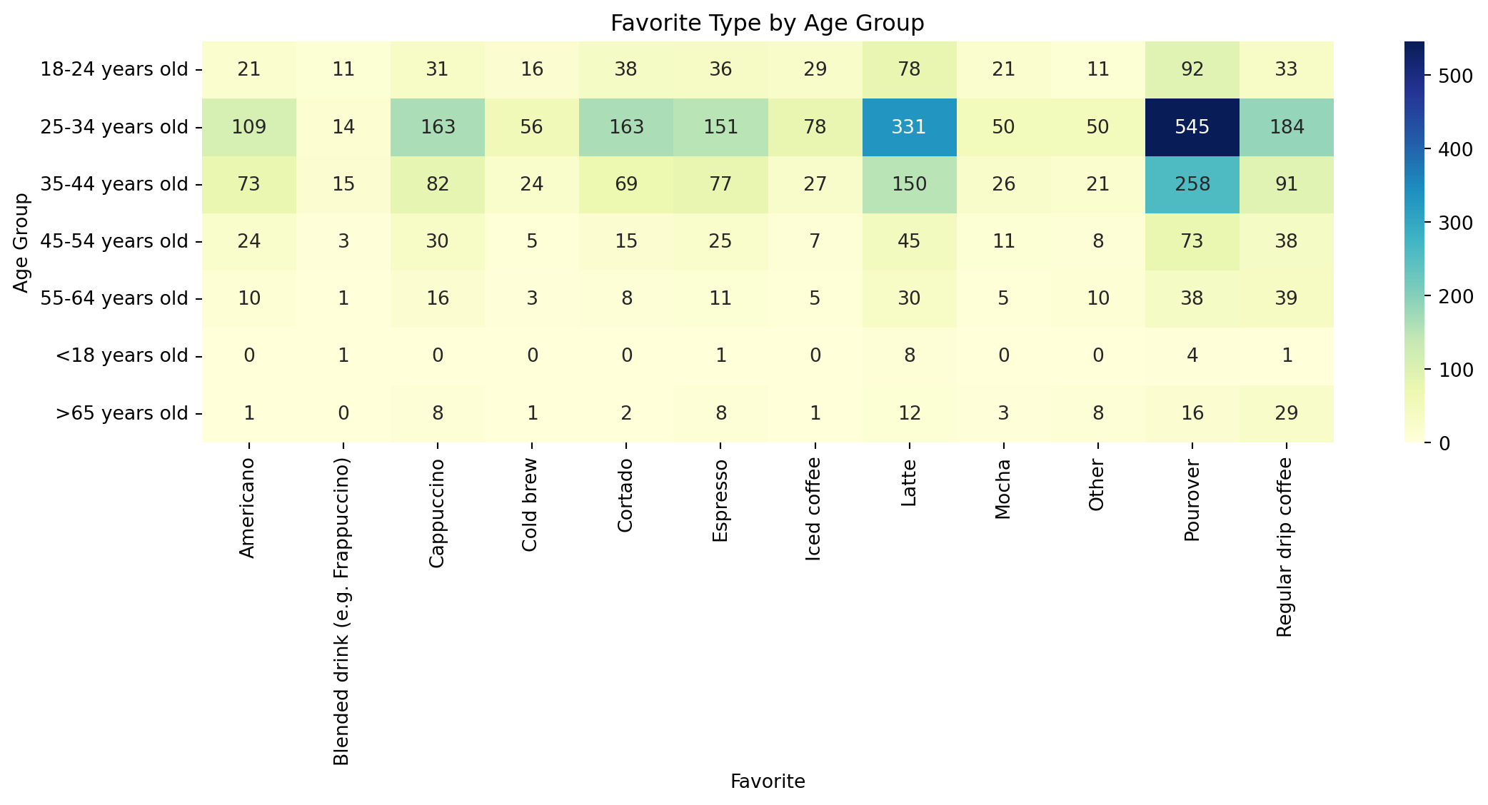

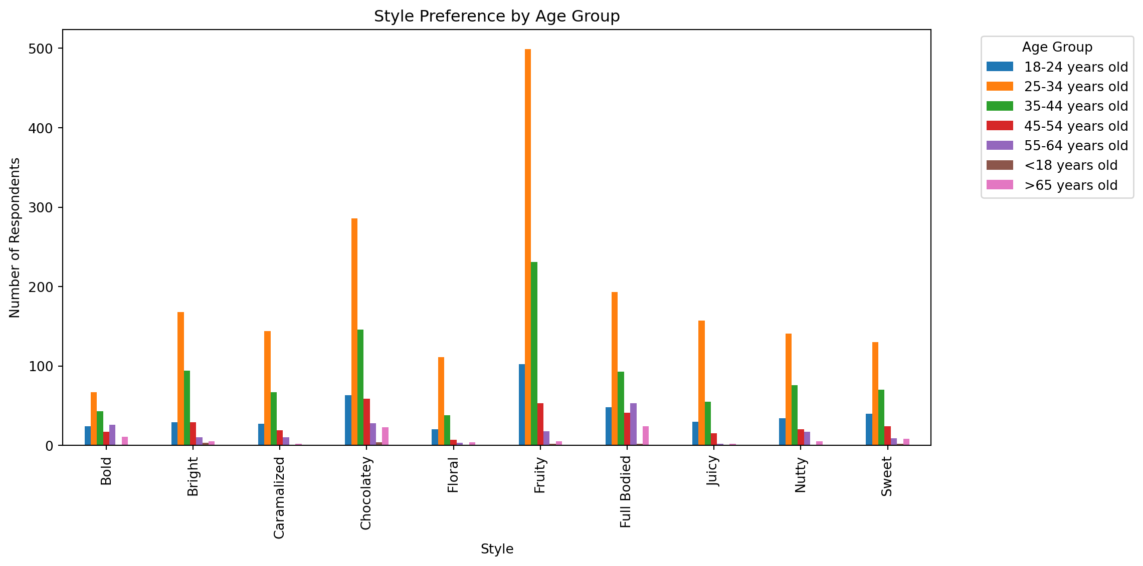
2.3 Preferred Style of Coffee by Age Group

#Group Style by Age

style_by_agegroup = df_focused.groupby('age')['style'].value_counts().unstack().fillna(0)

Grouped bar plt

style_by_agegroup.T.plot(kind='bar', figsize=(12, 6))
plt.title('Style Preference by Age Group')
plt.ylabel('Number of Respondents')
plt.xlabel('Style')
plt.legend(title='Age Group', bbox_to_anchor=(1.05, 1), loc='upper left')
plt.tight_layout()
plt.show()